Details: Written by Super User; Category: Design of Experiments (DOE) - Case Studies; Published: 16 March 2020

Introduction

This article will demonstrate how QLazDOE software can manage single-factor experiments with multiple levels (i.e. multiple treatments), using one-way ANOVA for analysis of results and driving conclusions.

Example used for this demonstration is from the book "Design and Analysis of Experiments" by Douglas C. Montgomery, which you can purchase from: https://www.wiley.com/en-hr/Design+and+Analysis+of+Experiments,+10th+Edition-p-9781119492443

Problem Statement

We will be dealing with a plasma etching process, where energy is supplied by a radio-frequency (RF) generator causing plasma to be generated in the gap between the electrodes. We are interested in investigating the relationship between the RF power setting and the etch rate for this tool. We want to determine whether etching rate depends on the RF power or not. We will test four levels of RF power: 160, 180, 200, and 220 W and measure etching rate as response variable. For each power settings, there will be 5 replicates.

This is a single factor experiment, with 4 levels (i.e. 4 treatments. Results will be analyzed by using one-way ANOVA. Null hypothesis H0 is that means for 4 treatments (i.e. power settings) are equal, while alternative hypothesis is that treatment means are different.

Definition of Factors and Levels

First we need to create new project, defining its name, description and problem statement.

Now we need to create factors & levels definition file. We can do it by clicking button or from corresponding menu item "Create New Factors and Levels Definition File" .

Design of Experiment

First we need to create new solution for the current project.

Now we will create our full factorial, replicated design of experiment, by clicking button or choosing corresponding option "Create DOE in one step" from the menu .

This creates and opens design of experiments in a spreadsheet, ready for results data input.

Experimental Results

Next is to conduct the experiment and enter experimental results. Our response variable is etching rate, so we need to add new column "Etching Rate" and enter results.

Analysis of Experimental Results

To analyze results, we need to load results into LazStats statistical software. We can do it by clicking on the button , or by choosing corresponding menu item "Analyze DOE Results in LazStats" . This opens LazStats with loaded results. Now we have to find ANOVA function under Analyses/Comparisons/1, 2, or 3 Ways ANOVAs.

ANOVA form opens, where we need to define Etch Rate as dependent (response) variable and RF Power as input factor with fixed levels.

Click the button "Compute" in order to acquire ANOVA results.

One-Way ANOVA

LazStats returns one-way ANOVA results as follows:

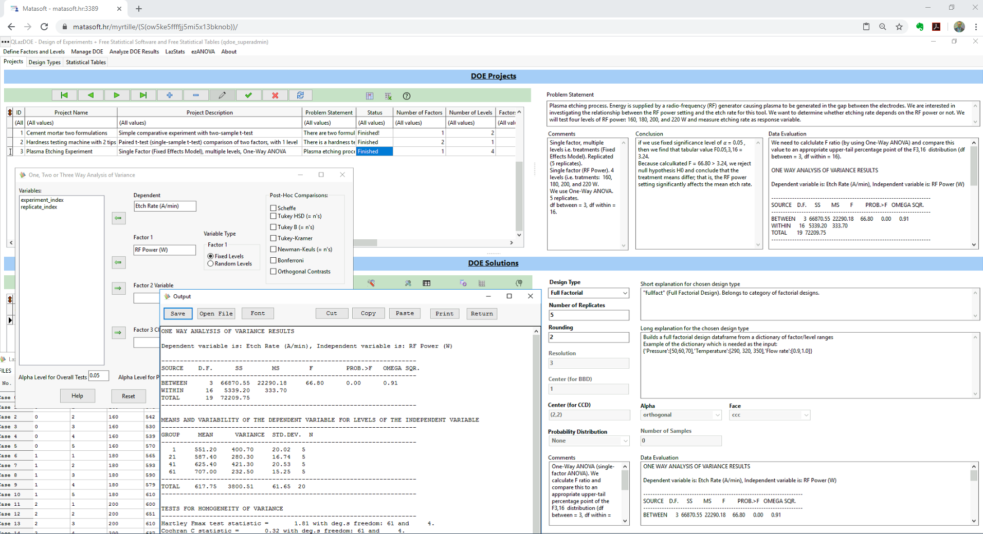
ONE WAY ANALYSIS OF VARIANCE RESULTS

Dependent variable is: Etch Rate (A/min), Independent variable is: RF Power (W)

---------------------------------------------------------------------
SOURCE D.F. SS MS F PROB.>F OMEGA SQR.
---------------------------------------------------------------------
BETWEEN 3 66870.55 22290.18 66.80 0.00 0.91
WITHIN 16 5339.20 333.70
TOTAL 19 72209.75
---------------------------------------------------------------------

MEANS AND VARIABILITY OF THE DEPENDENT VARIABLE FOR LEVELS OF THE INDEPENDENT VARIABLE
---------------------------------------------------------------------
GROUP MEAN VARIANCE STD.DEV. N
---------------------------------------------------------------------
1 551.20 400.70 20.02 5
21 587.40 280.30 16.74 5
41 625.40 421.30 20.53 5
61 707.00 232.50 15.25 5
---------------------------------------------------------------------
TOTAL 617.75 3800.51 61.65 20
---------------------------------------------------------------------

TESTS FOR HOMOGENEITY OF VARIANCE
---------------------------------------------------------------------
Hartley Fmax test statistic = 1.81 with deg.s freedom: 61 and 4.
Cochran C statistic = 0.32 with deg.s freedom: 61 and 4.
Bartlett Chi-square = 0.43 with 3 D.F. Prob. > Chi-Square = 0.933
---------------------------------------------------------------------

So, our calculated F-ratio statistics, F = 66.80. Now we need to compare it with tabular value for F distribution for degrees of freedom DF between = 3, DF within = 16.

Let's go to "Statistical Tables" tab and find F Distribution sub-tab.

If we use fixed significance level of alpha = 0.05 , then we find that tabular value F0.05,3,16 = 3.24.

Because F = 66.80 > 3.24, we reject H0 and conclude that the treatment means differ; that is, the RF power setting significantly affects the mean etch rate.

Graphical Visualization

It is always good idea to visually check numerical calculation before driving any conclusion. For example, we might use "Multiple Group X vs Y Plot" option in LazStats.

Building a Model (Regression)

One of the DOE purposes is to determine mathematical model of a process, i.e. to establish a mathematical formula by which one could predict response variables (process output) for a given set of input variables.

Integrated LazStats software has multiple options for performing regression. For purpose of this article, we will briefly show standard "Least Squares Multiple Regression". Go to Analyses/Multiple Regression/Least Squares Multiple Regression.

In the multiple regression parameters form, set Etch Rate as depndent variable and RF Power as independent variable. Click Compute button.

LazStats returns regression analysis with built model of our process.

We can see that the LazStats returned following linear model of our process: Y=137.620 + 2.527 X

Conclusion

If we use fixed significance level of alpha = 0.05 , then we find that tabular value F0.05,3,16 = 3.24.
Because calculated F = 66.80 > 3.24, we reject null hypothesis H0 and conclude that the treatment means differ; that is, the RF power setting significantly affects the mean etch rate!

Determined linear model of our process is Y=137.620 + 2.527 X, where Y= etching rate and X = RF power.

Also, P-value is smaller than 0.00, which also confirms our conclusion!

Appendix 1: Full Randomization

In many real-life DOE experiments it is important to ensure that experiment is performed in random order, so that the environment in which treatments are applied is as uniform as possible, i.e. that environmental fluctuations have minimal effect on conclusions.

To ensure completely randomized design, we can add a column into a DOE matrix spreadsheet, containing random numbers generated by LazStats. Then we can apply sorting on the column with random numbers, instead of default sorting by experiment index and replicate index.

First we need to open DOE matrix file and add new column for randomized numbers.

Then we have to generate random numbers in LazStats and copy generated values into the new column in DOE matrix.

Finally, we need to select all column ranges (without column headers) and apply sorting on the column with random numbers.

After sorting is applied, we have completely randomized DOE.

Appendix 2: More on Regression Analysis

Starting from version 1.0.2 QLazDOE has included simple regression function fitting program by which model for single factorial cases (one dependent response variable and one independent input variable) can be easily fitted. The program supports linear and non-linear regression (polynomial, exponential, power).

DOE resultset can be loaded into the regression program by clicking button or by choosing corresponding item menu "Simple Regression on DOE Results".

This will load data into the regression program and will open it in a separate form.

We can now choose independent (X) and dependent variable (Y).

We can also choose fitting equation and order (for polynomial equation).

Linear Regression

if we choose linear model, we will get exactly the same results as with LazStats regression.

Non-Linear (Polynomial) Regression

If we choose polynomial fitting function, for example of 2nd degree, we can see that the resulting model has better R-Squared value, meaning that the model better explains data than the linear model.

Therefore, this model would be the model of choice.

Of course, we might fit even higher polynomial models, but typically we would search for the simplest model explaining data well enough.

Plasma Etching Experiment (Example of Single Factor Experiment, Fixed Effects model, 4 Replicates, One-Way ANOVA)